Electric Charges and Fields Class 12 Notes Chapter 1 Physics

Table of Contents

In this article you will get NCERT and CBSE Physics Chapter 1 Electric Charges and Fields Class 12 notes. These have been prepared by the subject matter experts who have a teaching experience of more than 12 years at the senior secondary level.

Also Check: Class 11 waves notes pdf

Also Check: Motion in a straight line notes

NCERT Class 12 Physics Chapter 1 Physics Electric Charges and Fields Notes

The chapter is about electrostatics, the branch of physics that studies forces, fields, and potentials resulting from static charges. These notes are equally good for CBSE students as well.

Also Check: NCERT Solutions for Class 10 Science Acids Bases and Salts

Electrostatics

The branch of physics which deals with the study of charges at rest is known as Electrostatics.

The word, “electricity” is derived from a Greek word “elektron” which means “amber” (a resinous fossil found on the shore of the Baltic Sea).

When amber is rubbed with woolen cloth (fur), it acquires the property of attracting small pieces of paper, leaves, and dust. Same types of property can be seen when a comb is rubbed with dry hair.

The phenomenon of attractive property is known as electrification, and a substance is said to be charged or electrified. Thus, electrification of a substance, when rubbed with some suitable material, is said to have frictional or static electricity.

Electric Charge

In dry weather, a spark is produced by walking across certain types of carpet and then bringing one of the fingers near a metal doorknob, metal faucet, or even a person.

Multiple sparks can be produced when a sweater is pulled from the body or clothes from a dryer. These examples reveal that electric charge is present in our bodies, carpet, faucets, sweaters, and computers.

In fact, every object contains a vast amount of electric charge.

Definition: The intrinsic property of material objects that make it possible for them to exert electrical force and to respond to electric force is known as electric charge.

The SI unit of electric charge is coulomb (C), and it is a scalar quantity. It causes the electric force in matter.

Benjamin Franklin, an American physicist, states that the vast amount of charge in an object is usually hidden because the object contains two kinds of charge in equal amounts:

(a) Positive charge
(b) Negative charge

Franklin’s sign conventions say that:

Like charges repel each other.
Unlike charges attract each other.

Electroscope

It is a simple device that can be used to test the presence of electric charges.

Earthing

The phenomenon in which we bring a charged body in contact with the earth or ground, and all the excess charge on the charged body leaks to the earth is called grounding or earthing.

Basic Properties of Electric Charges

Definition of Point Charges

If the size of a charged body is very small as compared to its distance from all other surrounding objects of interest, then such a body can be considered as a point charge.

Additive Nature of Electric Charge

Electric charge is additive in nature. This means that if a system consists of two charges q1 and q2, then the total charge of the system will be:

$ q_{\text{total}} = q_1 + q_2 $

Similarly, if a system consists of three charges q1, q2, and q3, then the total charge of the system will be:

$ q_{\text{total}} = q_1 + q_2 + q_3 $

In general, if a system consists of n charges q1, q2, q3 ,q4, ..…, qn, then the total charges of the system will be:

$ q_{\text{total}} = q_1 + q_2 + q_3 + q_4 + \dots + q_n $

Since electric charge is a scalar quantity, in these examples, in order to calculate the net charge on a system, we have to add algebraically all the charges in the system. This shows that charge is additive in nature.

Conservation of Electric Charge

The law states that no positive or negative charge can either be created or destroyed by itself.

The charge may only be transferred from one body to another. In other words, in an isolated system, the total amount of charge remains constant.

In an experiment, if a positively charged particle is created, there must be the simultaneous creation of a negative charged particle of the same magnitude.

The sum total of charge before and after the experiment must be zero. We may also state that the universe as a whole is electrically neutral.

EXPERIMENTAL PROOF:

No exception has been found to the law of conservation of charge experimentally so far. The two cases of interest are:

i)In an experiment, if an electron (-e) and a positron (+e) are brought close to each other, they disappear and convert the whole rest mass into energy.

The process obeys the relation (E = mc^2) and is called annihilation. The product of the process is two gamma photons.

Electron (-e) + Positron (+e) → Photon (0 charge).

→ Net charge is zero before and after the process. Hence charge is conserved.

ii)In radioactive decay processes, the law of conservation of charge is always found to hold true.

\[{}^{92}\text{U}_{238} \rightarrow {}^{90}\text{Th}_{234} + {}^{2}\text{He}_{4}.\]

Net charge is zero before and after the process.

iii) In all nuclear reactions, the net algebraic sum of charges of reactant nuclei is the same as that of the product nuclei. The law of conservation of charge forms a basic principle in nuclear physics.

QUANTIZATION OF CHARGE

According to the quantization of charge, the charge on any object is always an integral multiple of the smallest unit of charge (e) and can be written as:

Q=ne

Where n is an integer and e is the basic or smallest unit of charge, which is equal to the charge on an electron.

The value of e is:

\[e = 1.6 \times 10^{-19} \, \text{C}.\]

The SI unit of charge is the coulomb (C), named after Charles Augustin de Coulomb, who studied electric forces in the late 1700s.

When a physical quantity such as charge can have only discrete values rather than any arbitrary value, we say that the quantity is quantized.

It is possible, for example, to find a free particle that has no charge at all or a charge of (+7e) or (-3e), but not a free particle with a charge of, say, (2.57e).

Modern studies of the structure of neutrons and protons have produced strong evidence that many particles are made up of tightly bound particles with charge ( +2e/3) and (-1e/3), that we call quarks, but quarks do not seem to exist as free particles. Hence fractional charges do not exist.

COULOMB’S LAW

The law was put forward by CHARLES AUGUSTIN DE COULOMB, a French physicist in 1785. This was the first quantitative law put forward for the force acting between the charged bodies at rest and marked an important step in the development of electrostatics. It is an electrostatic analogue of Newton’s Universal law of gravitation.

STATEMENT: It states that, “the force of interaction between any two point charges at rest is directly proportional to the product of the charges and inversely proportional to the square of the distance between them”.

The force acts along the line joining the two point charges. Let (q₁) and (q₂) are two point charges at rest separated by a distance (r) in vacuum or air. The point charges are small; approximation can be met if the charges are small in size as compared to the distance ‘r’ between them.

Mathematically:

\[ F \propto q_1 q_2 \]

\[ F \propto \frac{1}{r^2} \]

Combining the two proportionalities, we get:

\[ F \propto \frac{q_1 q_2}{r^2} \]

\[ \ or\ F = k \frac{q_1 q_2}{r^2} \]

Where (k) is the constant of proportionality and is called Coulomb’s electrostatic constant. It can be expressed as:

\[ k = \frac{1}{4 \pi \epsilon_0} \]

Experimentally, it is found that ( k ) is equal to $ 9 \times 10^9 \, \text{N·m}^2/\text{C}^2 $ in the SI system and (k = 1) in the CGS system.

ε₀is called the absolute permittivity of vacuum and is equal to 8.85×10^-12 C₂N^-1m².

Thus, the magnitude of force is:

\[ F = \frac{1}{4 \pi \epsilon_0} \frac{q_1 q_2}{r^2} \]

It is clear from the above expression that:

When both q₁ and q₂ are like charges, the force is positive and denotes a force of repulsion.
If the charges are of opposite sign, then the force is negative and denotes a force of attraction between them.

Since Coulomb’s law is an inverse square law, the same as the gravitational force, but electrostatic forces are stronger than gravitational forces.

Coulomb’s law has been verified to hold true over distances from 10^-15m to several kilometers. At distances r < 10^-15m , the nuclear forces become dominant.

POINT TO BE REMEMBERED

The ability of a substance to store electrical energy in an electric field gives us permittivity of that substance.
Permittivity is a measure of how an electric field affects and is affected by a medium.
SI unit of charge is coulomb.
CGS unit of charge is stat coulomb or e.s.u. (electrostatic unit).
Electromagnetic unit is absolute coulomb (ab coulomb).
Relationship:

$$1 \, \text{coulomb} = 3 \times 10^9 \, \text{stat coulomb}$$

and

$$1 \, \text{coulomb} = \frac{1}{10} \, \text{ab coulomb}.$$

COULOMB’S LAW IN VECTOR FORM or COULOMB’S LAW IN ACCORDANCE WITH THE NEWTON’S THIRD LAW OF MOTION

Let us consider two point charges (q₁) and (q₂) placed at (A) and (B) in vacuum.

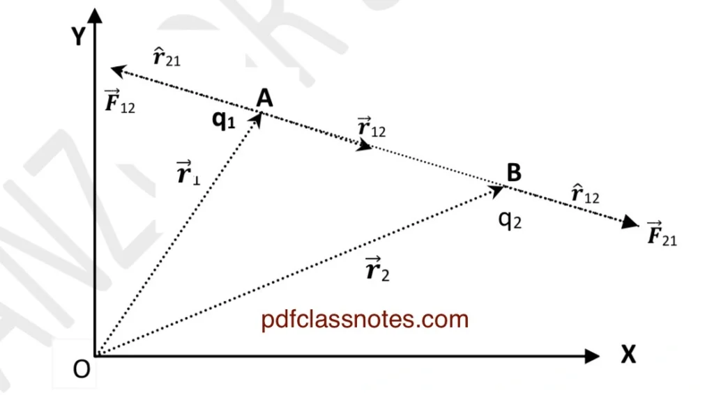
Let $ \vec{r_1} $ and $ \vec{r_2} $ be their position vectors with respect to the origin.

Using the triangle law of vector addition in (△ OAB ):

$$\overrightarrow{OA} + \overrightarrow{AB} = \overrightarrow{OB}$$

$$\overrightarrow{AB} = \overrightarrow{OB} – \overrightarrow{OA} = \vec{r_2} – \vec{r_1}.$$

Let us denote:

$$\vec{r_2} – \vec{r_1} = \vec{r_{12}}.$$

Let us denote $ \vec{F_{21}} $ as the force on charge $ q_2 $ due to $ q_1 $. Similarly, $ \vec{F_{12}} $ will mean the force on charge $ q_1 $ due to $ q_2 $. This symbolism is a mere convention.

Now the force on (q₁) due to (q₂) will be expressed as:

$$\vec{F_{12}} = \frac{1}{4 \pi \varepsilon_0} \frac{q_1 q_2}{r_{12}^2} \hat{r_{21}}.$$

The direction of the unit vector $ \hat{r_{21}} $ is shown along $ \overrightarrow{BA} $.

Similarly, the force on (q₂) due to (q₁) will be expressed as:

$$\vec{F_{21}} = \frac{1}{4 \pi \varepsilon_0} \frac{q_1 q_2}{r_{12}^2} \hat{r_{12}}.$$

The direction of the unit vector $ \hat{r_{12}} $ is shown along $ \overrightarrow{AB} $ in the figure.

Since $$\hat{r_{12}} = -\hat{r_{21}}.$$

$$\vec{F_{21}} = \frac{1}{4 \pi \varepsilon_0} \frac{q_1 q_2}{r_{12}^2} \cdot (-\hat{r_{21}}) = -\vec{F_{12}}.$$

Thus, electrostatic forces are mutual forces which obey Newton’s third law of motion.

FORCE DUE TO MULTIPLE CHARGES

(PRINCIPLE OF SUPERPOSITION)

The electrostatic force obeys the principle of superposition. This principle is just the polygon law of force in mechanics. This principle enables us to obtain total force on a given charge due to any number of point charges or continuous charge distribution.

The principle of superposition states that, “the total force on a given charge due to a number of point charges is equal to the vector sum of the individual forces exerted by the individual charges on the given charge”. Each individual force is calculated from Coulomb’s law and is not affected by the presence of other charges.

Let us consider a group of discrete charges (q1), (q2), (q3), …, (qn) situated at different points with the position vectors $ \vec{r}_1, \vec{r}_2, …, \vec{r}_n $ respectively with respect to the origin as shown in the figure.

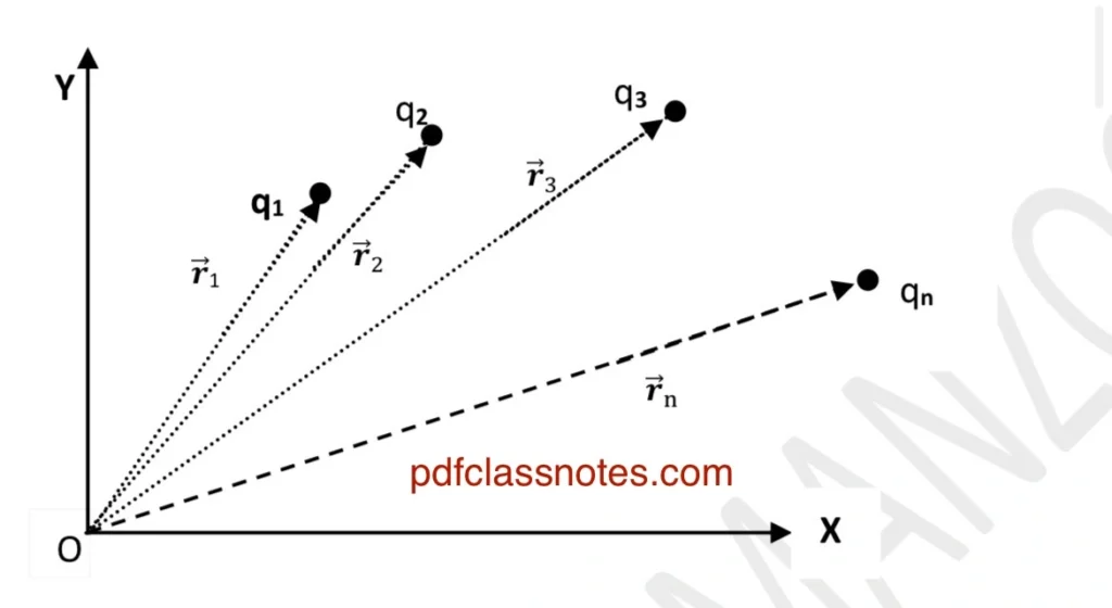
The principle of the superposition gives the following method of determining the total force (F₁), which will act on the charge (q₁) due to the whole set of charges:

(1) We first compute the force $ \vec{F}_{12} $ on $ \ q_1 $ due to $ \ q_2 $ alone. We do so by ignoring all other charges as if they were not present.

(2)Then we compute the force $ \vec{F}_{13} $ on $ \ q_1 $ due to $ \ q_3 $ by ignoring the presence of all other charges.

(3) Similarly, we compute the forces $ \vec{F}_{14}, \vec{F}_{15}, …, \vec{F}_{1n} $. To compute these individual forces, we use Coulomb’s law.

(4) Finally, the resultant force $ \vec{F}_1 $ on charge $ \ q_1 $ is given by the vector sum of all the individual forces acting on $ \ q_1 $ due to $ \ q_2, q_3, …, q_n$.

\[ \vec{F}_1 = \vec{F}_{12} + \vec{F}_{13} + \vec{F}_{14} + \dots + \vec{F}_{1n} \]

The procedure stated above is called the principle of superposition.

\[ \vec{F}_1 = \frac{1}{4 \pi \epsilon_0} \frac{q_1 q_2}{r_{21}^2} \hat{r}_{21} + \frac{1}{4 \pi \epsilon_0} \frac{q_1 q_3}{r_{31}^2} \hat{r}_{31} \\ + \frac{1}{4 \pi \epsilon_0} \frac{q_1 q_4}{r_{41}^2} \hat{r}_{41} + \dots + \frac{1}{4 \pi \epsilon_0} \frac{q_1 q_n}{r_{n1}^2} \hat{r}_{n1} \]

Where,

\[ \hat{r}_{21} = \frac{\vec{r}_2 – \vec{r}_1}{|\vec{r}_2 – \vec{r}_1|} \quad \hat{r}_{31} = \frac{\vec{r}_3 – \vec{r}_1}{|\vec{r}_3 – \vec{r}_1|} \quad \text{and so on.} \]

\[ \vec{F}_1 = \frac{1}{4 \pi \epsilon_0} \frac{q_1 q_2}{r_{21}^2} \hat{r}_{21} + \frac{1}{4 \pi \epsilon_0} \frac{q_1 q_3}{r_{31}^2} \hat{r}_{31} \\ + \dots + \frac{1}{4 \pi \epsilon_0} \frac{q_1 q_n}{r_{n1}^2} \hat{r}_{n1} \]

\[ \ or \vec{F}_1 = \frac{1}{4 \pi \epsilon_0} \sum_{i=1}^n \frac{q_1 q_i}{r_{i1}^2} \hat{r}_{i1} \]

DIELECTRIC CONSTANT OR RELATIVE PERMITTIVITY

The electrostatic force of attraction or repulsion between two charges is influenced by the intervening medium between them.

The extent to which a medium like water, glass, mica, or any other material medium affects the electrostatic force is expressed by stating the value of the dielectric constant of that medium.

We compare the force between two given charges by placing vacuum between them with that force which they have when a medium other than vacuum or air is placed between them.

The ratio of the two forces gives the dielectric constant of the medium.

Let, (F₀) be the force of attraction or repulsion between two charges when they are placed in vacuum.

\[ |F_0| = \frac{1}{4 \pi \epsilon_0} \frac{q_1 q_2}{r^2} \tag{1} \]

Where (ε₀) is an intrinsic property of vacuum called its absolute electric permittivity.

Let (F_m) be the new value of force between the same charges at the same distance when placed in a medium other than vacuum.

\[ k = \frac{1}{4 \pi \epsilon_0} \text{ is replaced by } \frac{1}{4 \pi \epsilon_m},\\ \text{ where } \epsilon_m \text{ is called the absolute permittivity of the medium.} \]

\[ \therefore |F_m| = \frac{1}{4 \pi \epsilon_m} \frac{q_1 q_2}{r^2} \tag{2} \]

Dividing equation (1) by equation (2):

\[ \frac{|F_0|}{|F_m|} = \frac{1}{4 \pi \epsilon_0} \frac{q_1 q_2}{r^2} \times \frac{4 \pi \epsilon_m r^2}{q_1 q_2} \]

\[ \frac{|F_0|}{|F_m|} = \frac{\epsilon_m}{\epsilon_0} \tag{3} \]

The ratio $ \frac{|F_0|}{|F_m|} $ is called the dielectric constant ($ K $) of the medium.

\[ \text{Dielectric Constant } K = \frac{\text{force between charges with vacuum between them}}{\text{force between charges with medium between them}} \]

\[ \text{or } K = \frac{|F_0|}{|F_m|} \\ \implies |F_m| = K^{-1} |F_0| \]

For water ( K = 80 ), it means that the presence of water between two charges will decrease the force between them by a factor of 80.

\[ F_\text{vacuum} = 80 \times F_\text{water} \]

CONTINUOUS CHARGE DISTRIBUTION

A system of closely spaced charges is said to form a continuous charge distribution. It does not mean that electric charge is continuous or charge is no longer discrete. It simply means that the distribution of discrete charges is continuous, with little space between the charges.

There are three kinds of continuous charge distribution:

1. Linear Charge Distribution:

When the charge is distributed uniformly along a line (e.g., a straight line or circumference of a circle), the linear charge density denoted by λ is equal to charge per unit length.

\[ \lambda = \frac{dq}{dl} \]

It is measured in (Cm^-1).

To calculate the total force (F) on a test charge (q₀) due to linear charge distribution, we consider a small element of length ( dl ) of the line ( L ).

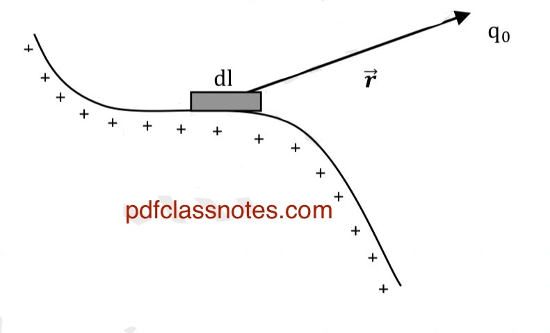
The small amount of charge on this element is:

\[ dq = \lambda dl \]

The force on (q₀) due to this charge element is:

\[ d\vec{F} = \frac{1}{4 \pi \epsilon_0} \frac{q_0 dq}{r^2} \hat{r} = \frac{q_0 \lambda dl}{4 \pi \epsilon_0 r^2} \hat{r} \]

When we add up all such contributions of the small charge elements vectorially, we get the total force on test charge (q₀) as:

\[ \vec{F} = \int_L \frac{q_0 \lambda dl}{4 \pi \epsilon_0 r^2} \hat{r} = \frac{q_0}{4 \pi \epsilon_0} \int_L \frac{\lambda dl}{r^2} \hat{r} \]

2. Surface Charge Distribution:

When the charge is distributed continuously over some area or a membrane, the distribution is known as surface charge distribution.

Let (σ) be the surface charge density, which is equal to charge per unit area:

\[ \sigma = \frac{dq}{ds} \]

The SI unit of σ is Cm^-2.

Let (ds) be a small surface on surface (S) as shown. Let a test charge (q₀) be placed in the vicinity of the surface charge distribution such that the distance between the test charge and the surface (ds) is (r).

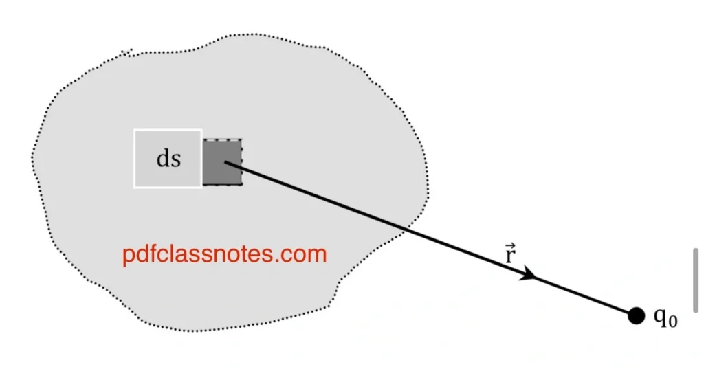
The force on (q₀) due to (dq) is expressed as:

\[ d\vec{F} = \frac{1}{4 \pi \epsilon_0} \frac{q_0 dq}{r^2} \hat{r} = \frac{q_0}{4 \pi \epsilon_0} \frac{ds}{r^2} \hat{r}. \]

Therefore, the total force on (q₀) due to the entire surface distribution of charge can be calculated by integrating the above expression:

\[ \vec{F} = \int_S \frac{q_0 \sigma ds}{4 \pi \epsilon_0 r^2} \hat{r} = \frac{q_0}{4 \pi \epsilon_0} \int_S \frac{\sigma ds}{r^2} \hat{r}. \]

3. Volume Charge Distribution:

Volume charge distribution refers to the uniform distribution of charge over a particular volume. The volume charge density is defined as the charge per unit volume of the volume charge distribution. It is represented by (ρ) as:

\[ \rho = \frac{dq}{dv} \]

The SI unit of volume charge distribution is (Cm^-3).

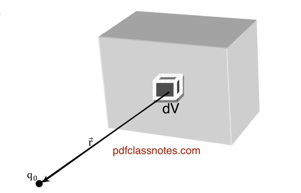
Let (dv) be a small volume on the given volume distribution. The charge (dq) on the volume (dv) is:

\[ dq = \rho \, dv. \]

Let a test charge (q₀) be placed in the vicinity of the volume charge distribution. The force on (q₀) due to (dq) is expressed as:

\[ d\vec{F} = \frac{1}{4 \pi \epsilon_0} \frac{q_0 dq}{r^2} \hat{r} = \frac{q_0}{4 \pi \epsilon_0} \frac{\rho \, dv}{r^2} \hat{r}. \]

Therefore, the total force on (q₀) due to the entire volume distribution of charge can be calculated by integrating the above expression:

\[ \vec{F} = \int_V \frac{q_0 \rho \, dv}{4 \pi \epsilon_0 r^2} \hat{r} = \frac{q_0}{4 \pi \epsilon_0} \int_V \frac{\rho \, dv}{r^2} \hat{r}. \]

ELECTRIC FIELD

Electric field may be defined as the space surrounding a charge or a system of charges within which the influence of these charges can be felt.

To feel the effect of a given electric field at a point, we use a very small electric charge (q₀), called as the test charge. The magnitude of force experienced by the test charge at a certain distance from the system of charges gives us an idea of the strength or intensity of the electric field at that point.

TEST CHARGE (DEFINITION): A test charge is a charge having magnitude so small that placing it at a point has a negligible effect on the field around the point. The direction of (E) is the same as that of the force on the positive test charge; directly away from the point charge if (q) is positive and towards it, if (q) is negative.

ELECTRIC FIELD STRENGTH OR INTENSITY

The electric field strength (E) may be defined as the force (F) acting on a positive charge placed in the field at the given point divided by the magnitude of charge (q₀).

\[ \vec{E} = \frac{\vec{F}}{q_0} \tag{1} \]

E has the same direction as that of the electric force F. The charge (q₀) should be very small so that it does not disturb the system of charges whose electric field is being determined.

\[ \vec{E} = \lim_{q_0 \to 0} \frac{\vec{F}}{q_0} \tag{2} \]

Substituting the expression for $ \vec{F} $:

\[ \vec{E} = \frac{1}{4 \pi \epsilon_0} \frac{q q_0}{r^2} \hat{r} \times \frac{1}{q_0} = \frac{1}{4 \pi \epsilon_0} \frac{q}{r^2} \hat{r} \tag{3} \]

The SI unit of $ \vec{E} $ is newton/coulomb, i.e., $ \text{NC}^{-1} $, or volt/meter (V/m).

Its dimensional formula is:

\[ [E] = [M^1 L^1 T^{-3} A^{-1}] \]

ELECTRIC FIELD LINES

Michael Faraday introduced the idea of the electric fields in the 19th century. It was thought that the space around a charged body is filled with the lines of force, now called electric field lines.

Presently, the reality of these lines is no longer considered valid, although they provide a nice way to visualize patterns in the electric field.

A line of force may be defined as an imaginary line, the tangent to which gives the direction of electric field intensity at that point. The following definitions give the relation of the electric field strength to the lines of force:

a) The electric field lines begin from positive charge and terminate or end on a negative charge.

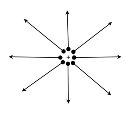
b) The tangent to a line of force at any point gives the direction of electric field at that point.

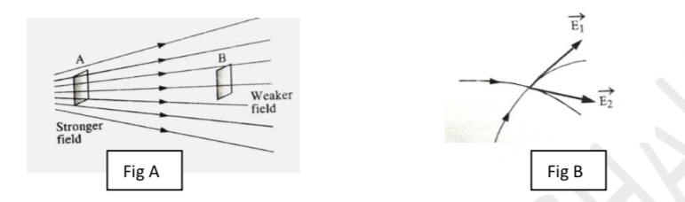
c) The magnitude of electric field is proportional to the number of lines crossing a unit area, which is held at normal to the direction of the field. Hence the lines are closely packed in regions of strong fields and are wider apart in the regions of weak fields (fig A).

d) Two electric lines of force do not cross each other. If two electric field lines cross each other, then there will be two tangents at the point of intersection (fig B). It means that there are two directions of the electric field at the same point, which is not possible. Hence no two electric field lines cross each other.

ELECTRIC DIPOLE

A system of two equal and opposite charges separated by a small distance forms an electric dipole.

Examples of electric dipoles are HCl, HF, H₂O, etc. Below, the figure shows an electric dipole that consists of two charges (+q) and (-q) separated by a very small distance (2a). Here (2a) is known as dipole length and is equal to the separation between the two charges of the electric dipole.

The dipole length (2a) is a vector quantity whose direction is from the negative charge towards the positive charge.

A molecule of water H₂O is an electric dipole. In a water molecule, the two hydrogen atoms and the oxygen atom do not lie on a straight line but form an angle of about 105° as shown in the figure.

As a result, the molecule has a definite oxygen and hydrogen side. Moreover, the ten electrons of the molecule tend to remain closer to the oxygen nucleus than to the hydrogen nuclei. This makes the oxygen side of the molecule slightly more negative than the hydrogen side and creates an electric dipole.

ELECTRIC DIPOLE MOMENT

The strength of an electric dipole is measured by a quantity that is called the electric dipole moment. The electric dipole moment is a vector quantity, and mathematically it is equal to the product of the magnitude of either of the charges and the dipole length, i.e.,

\[ \vec{p} = |q| \times 2a \]

Here, $ \vec{p} $ is the electric dipole moment, $ |q| $ is the magnitude of either of the charges, and $ 2a $ is the dipole length.

The SI unit of dipole moment is coulomb meter (Cm). The dipole moment is also a vector quantity and is directed towards the positive charge from the negative charge.

ELECTRIC DIPOLE FIELD

The electric field of an electric dipole may be defined as the space around the dipole in which the electric effect of the dipole can be experienced.

An electric dipole consists of two charges (+q) and (-q); therefore, according to the principle of superposition, the electric field due to an electric dipole at a point will be equal to the vector sum of the electric field due to the two individual charges.

For simplicity, we will find the electric field due to an electric dipole only on two lines:

Axial Line
Equatorial Line

1. Electric field intensity at a point on the axial line of the dipole:

Definition: A line joining the centers of the two charges of an electric dipole is known as the axial line of the electric dipole. Let us consider an electric dipole consisting of two point charges (+q) and (-q) separated by a distance (2a) between them.

Let ‘P’ be the point on the axis of the dipole at a distance (r) from the center of the dipole, as shown in the figure below. O is the center of the dipole.

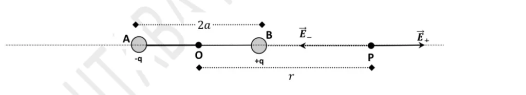
Let $ \vec{E}_+ $ be the intensity of the electric field at point $ P $ due to the charge $ +q $ and is directed along $ AP $:

\[ |\vec{E}_+| = \frac{1}{4 \pi \epsilon_0} \frac{q}{AP^2} = \frac{q}{4 \pi \epsilon_0 (r + a)^2} \tag{1} \]

Let $ \vec{E}_- $ be the intensity of the electric field at point $ P $ due to the charge $ -q $. The charge $ -q $ attracts the test charge $ q_0 $ at point $ P $ and is directed along $ PB $ to the left of $ P $.

\[ |\vec{E}_-| = \frac{1}{4 \pi \epsilon_0} \frac{q}{PB^2} = \frac{q}{4 \pi \epsilon_0 (r – a)^2} \tag{2} \]

The vectors $( \vec{E}+ $ and $( \vec{E}- $ are two collinear vectors acting in opposite directions. From equations (1) and (2), it is clear that $( |\vec{E}-| > |\vec{E}+| $. The magnitude of the resultant intensity at point (P) is given as:

\[ |\vec{E}_\text{net}| = |\vec{E}_-| – |\vec{E}_+| \]

Electric Field at a Point on the Axial Line of a Dipole

It is the expression for the magnitude of electric charge field intensity at point ‘P’ due to the dipole.

Since the negative charge (-q) is closer to the point (P), the direction of (E) at point (P) is towards (-q), i.e., along ( PB ).

$$ |\mathbf{E}_{\text{axial}}| = |\mathbf{E}_{+} – \mathbf{E}_{-}| \ $$

Substituting the values of E₊ and E_–from above, we get,

$$ |\mathbf{E}_{\text{axial}}| = \left| \frac{q}{4\pi\epsilon_0(r-a)^2} – \frac{q}{4\pi\epsilon_0(r+a)^2} \right| $$

$$ \Rightarrow |\mathbf{E}_{\text{axial}}| = \frac{q}{4\pi\epsilon_0} \left[ \frac{1}{(r-a)^2} – \frac{1}{(r+a)^2} \right] $$

$$ \Rightarrow |\mathbf{E}_{\text{axial}}| = \frac{q}{4\pi\epsilon_0} \cdot \frac{(r+a)^2 – (r-a)^2}{(r+a)^2(r-a)^2} $$

$$ \Rightarrow |\mathbf{E}_{\text{axial}}| = \frac{q}{4\pi\epsilon_0} \cdot \frac{4ar}{(r^2-a^2)^2} $$

$$ \Rightarrow |\mathbf{E}_{\text{axial}}| = \frac{2aq}{4\pi\epsilon_0} \cdot \frac{2r}{(r^2-a^2)^2} $$

The magnitude of the dipole moment is:

$$ |\mathbf{p}| = 2a \cdot |q| $$

Therefore, we can write;

$$ |\mathbf{E}_{\text{axial}}| = \frac{|\mathbf{p}|}{4\pi\epsilon_0} \cdot \frac{2r}{(r^2-a^2)^2} $$

This is the expression for the magnitude of the electric charge field intensity at point ‘P’ due to the dipole.

Since the negative charge (-q) is closer to the point (P), the direction of (E) at point (P) is towards (-q), i.e., along (PB).

Special Case:

For a short dipole 2a<r, point ‘P’ is at a distance (r), which is much larger than the distance (2a) between (+q) and (-q). We can ignore a² against r² in such cases.

$$ |\mathbf{E}_{\text{axial}}| = \frac{|\mathbf{p}|}{4\pi\epsilon_0 r^2} \cdot \frac{2r}{r^2} $$

$$ |\mathbf{E}_{\text{axial}}| = \frac{2|\mathbf{p}|}{4\pi\epsilon_0 r^3} $$

Electric Field at a Point on the Equatorial Line of a Dipole

Definition:

A line that is perpendicular to the axial line and passes through the center of an electric dipole is known as the equatorial line of the electric dipole.

Let us consider an electric dipole consisting of two-point charges (+q) and (-q) separated by a distance (2a) between them.

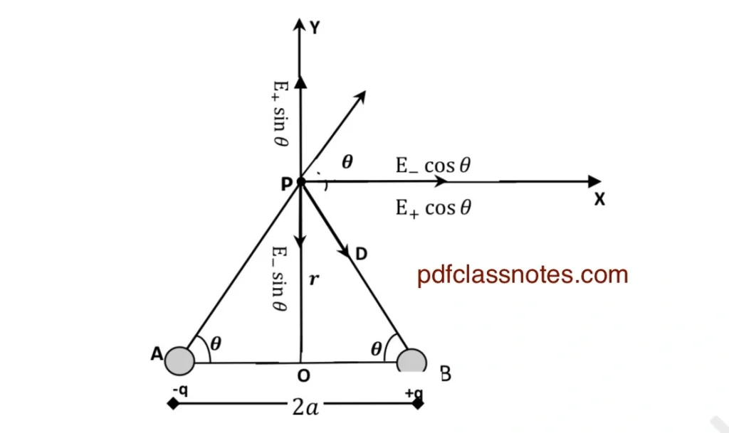
Let ‘P’ be the point on the equatorial line of the dipole at a distance (r) from the center (O) of the dipole as shown in the figure below.

Let ( OP = r ). Let $( \mathbf{E}_{+} $ be the electric field intensity at point ( P ) due to charge ( +q ), and its magnitude and direction are represented by the vector $ \vec{PC} $.

$$ |\mathbf{E}_{+}| = \frac{1}{4\pi\epsilon_0} \cdot \frac{q}{AP^2} —(1)$$

Using Pythagoras theorem, we can write

$$ AP^2 = PB^2 = a^2 + r^2 \quad \ $$

Using this value of (AP)² in (1), we get

$$ |\mathbf{E}_{+}| = \frac{q}{4\pi\epsilon_0 (a^2 + r^2)} $$

Now let $ \vec{E}{-} $ be the electric field intensity at point (P) due to charge (-q). Due to the attraction between charge (-q) and test charge $ (q_0) $ at ‘P,’ $ \vec{E}{-} $ is directed along (PB). Let $ \vec{PD} $ represent $ \vec{E}{-} $ in magnitude and direction.

$$ |\mathbf{E}_{-}| = \frac{q}{4\pi\epsilon_0 PB^2} = \frac{q}{4\pi\epsilon_0 (a^2 + r^2)} $$

To find the resultant electric field at (P), we resolve $ \vec{E}{+} $ and $ \vec{E}{-} $ into rectangular components along the (x)-axis and (y)-axis at point (P). Let $ \angle PAB = \theta $.

Resultant Electric Field Components:

$ \ E_+ \sin\theta $: Vertical component of $ \mathbf{E}_{+} $ along (PY).

$ \ E_+ \cos\theta $: Horizontal component of $ \mathbf{E}_{+} $ along (PX).

Also:

$ \ E_- \sin\theta $: Vertical component of $ \mathbf{E}_{-} $ along (PB).

$ \ E_- \cos\theta $: Horizontal component of $ \mathbf{E}_{-} $ along (PX).

The vertical components $ \ E_+ \sin\theta $ and $ \ E_- \sin\theta $ lie in opposite directions and are equal in magnitude. Hence, they cancel each other.

$$ Further |\mathbf{E}_+| = |\mathbf{E}_-| = |\mathbf{E}| $$

Resultant Intensity:

$$ \mathbf{E}_{\text{resultant}} = |\mathbf{E}_{+}| \cos\theta + |\mathbf{E}_{-}| \cos\theta $$

$$ \mathbf{E}_{\text{resultant}} = 2|\mathbf{E}| \cos\theta $$

Substituting:

$$ |\mathbf{E}_{\text{equatorial}}| = \frac{1}{4\pi\epsilon_0} \cdot \frac{2q}{(a^2 + r^2)^{3/2}} \cdot a $$

Special Case: For short dipole (2a<r). Point ‘P’ is at a distance which is much larger than the distance (2a) between (+q) and (-q). We may ignore (a²) against (r²) in such a case.

$$ \therefore \lvert \mathbf{E}_{\text{Equitorial}} \rvert = \frac{\lvert \mathbf{p} \rvert}{4\pi \epsilon_0 r^3} \implies \lvert \mathbf{E} \rvert \propto \frac{1}{r^3} $$

Electric dipole in the uniform electric field | Torque acting on the dipole in the uniform electric field

“Torque due to force gives us the turning effect of the force about the fixed point or axis.”

Let us consider an electric dipole of dipole moment (P) placed in an external electric field (uniform) of intensity (E). The dipole consists of charges (+q) and (-q) separated by a distance (2a). These charges experience equal and opposite forces in the field given by:

$$ \mathbf{F} = q \mathbf{E} \tag{1} $$

There is no tendency of linear motion because the net linear force on the dipole is zero. But the two equal and opposite forces (+F) and (-F) form a couple which tends to rotate the dipole. The turning effect of the couple is given by its torque (𝜏).

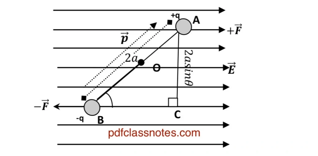
The axis of rotation of the electric dipole passes through (O) and is perpendicular to the plane containing the charges. (P) makes an angle (θ) with the field (E). The magnitude of torque on the electric dipole can be calculated by using the relation:

$$ \boldsymbol{\tau} = \text{magnitude of either force} \times \\ \text{perpendicular distance b/w the forces} $$

The perpendicular distance between the two forces is given by AC and its value can be found from (△ABC).

$$ \boldsymbol{\tau} = \text{F} \times \text{AC} \tag{2} $$

Now In △ABC,

$$ \sin \theta = \frac{AC}{AB} $$

$$ \Rightarrow AC = 2a \sin \theta \tag{3} $$

Substituting values from equations (1) and (3) in (2), we get

$$ \boldsymbol{\tau} = qE \times 2a \sin\theta $$

$$ \ or\ \boldsymbol{\tau} = (q \times 2a) \times E \times \sin \theta = pE \sin \theta \\ \implies \boldsymbol{\tau} = pE \sin \theta $$

We can generalize this equation to vector form as:

$$ \boldsymbol{\tau} = \ ( \vec{p} \ ) \times \ ( \vec{E} \ ) $$

The direction of (𝜏) is perpendicular to the plane containing (P) and (E).

The torque (𝜏) is maximum in magnitude when (θ = 90 degree) and 𝜏= 0 When (θ = zero), hence the torque acting on the dipole will always tend to align the dipole in the direction of the electric field.

So, these were NCERT and CBSE Physics Chapter 1 Electric Charges and Fields Class 12 notes. We are sure that you loved these Physics notes.